Microwave Circuits and Metamaterials

Project 8

Overview

Remain in same project groups for the semester.

The objective of this project is to simulate coaxial lines using HFSS software.

NOTE: Use the Project Report Template and keep answers to questions on consecutive sheets of paper with all plots at the end.

IN NO CASE may code or files be exchanged between students, and each student must answer the questions themselves and do their own plots, NO COPYING of any sort! Nevertheless, students are encouraged to collaborate in the lab session.

Only turn in requested plots ( Pxx ) and requested answers to questions ( Qxx ).

Part 1

In this part, you will simulate coaxial lines using HFSS software.
Impedance and phase characteristics will be determined.

Load and run the pulse example as follows:

Run HFSS from the linux window menu using Mosaic::Engineering::Electrical::HFSS
If this is the first time you run the software, make a note of the location of the default directory that will be created for your projects
Store all projects in this directory
Download the following zip-file (you may need to hold down the shift key while you click on the link):
mwMetaProj8a.hfss
Move the file into the HFSS directory
Load the project from within HFSS using MenuBar::File::Open (red circle below)

Double-click the "coaxAirWaveport1" design (upper left red arrow below), and select the copper cylynder2 (middle red arrow below), to see the corresponding 3D model (upper right red arrow below)

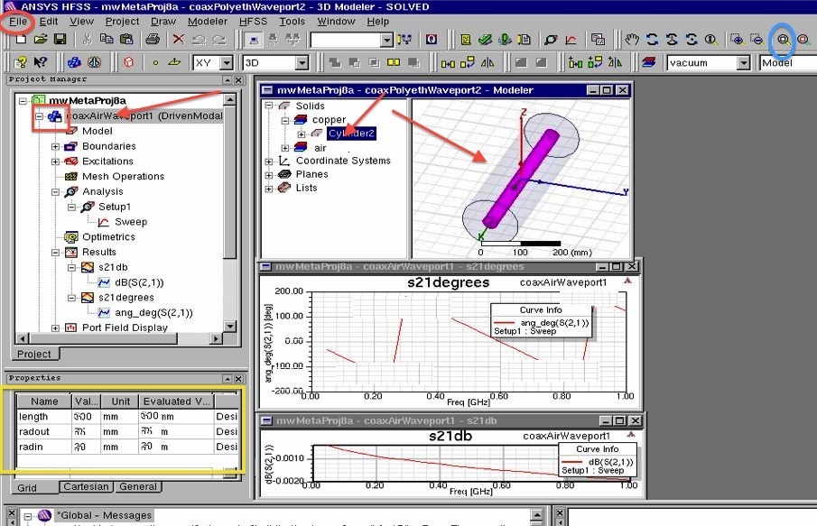
Press the fitAll button (blue circle above), if the entire 3D model is not visible
When you select the cylinder2 item (middle red arrow above), the corresponding 3D cylinder is highlighted
Save a snapshot of the 3D model and paste it into your report. ( P1 )
Make sure that your plots, component values, legends, axes, and fonts are legible in your report!
Click the "coaxAirWaveport1" design icon (upper left red box above) to see the variables used in the design (lower left yellow box)
From the variables, what is the length of the coaxial line? ( Q1 )
From the variables, what is the radius of the inner conductor of the coaxial line? ( Q2 )
From the variables, what is the radius of the outer conductor of the coaxial line? ( Q3 )
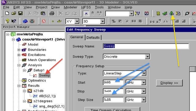
Double-click the analysis setup icon (red arrow below) to observe the setup for the 3D solver

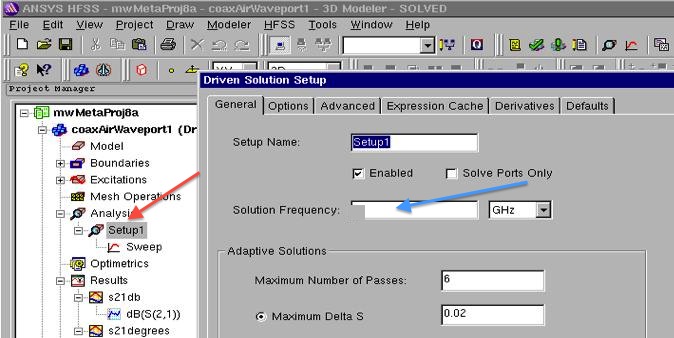
From the analysis setup, what is solution frequency (blue arrow above)? ( Q4 )
Double-click the analysis setup icon (red arrow below) to observe the setup for the 3D solver

From the sweep setup, what are start and stop frequencies (blue arrows above)? ( Q5 )
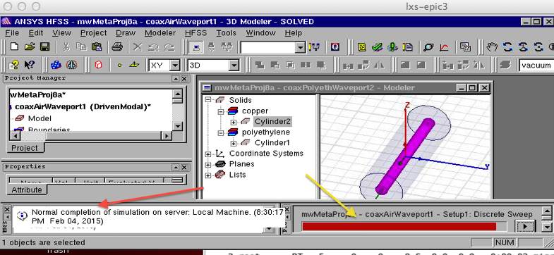
Run the simulation (yellow arrow above)
In the bottom right, during any simulation, you will see a progress bar (yellow arrow below)

If your project runs successfully, you should get a message (red arrow above) such as

[info] Normal completion of simulation on server: Local Machine. (8:30:17 PM Feb 04, 2035)

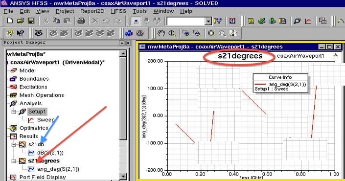
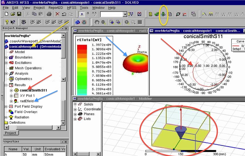
Observe the phase of S21 in degrees by double-clicking the Results::s21degrees (red arrow below)

Save a snapshot of the plot of the angle of S21 in degrees (yellow rectangle above with heading in red circle ) and paste it into your report. ( P2 )
At what frequency is the coaxial line section 90 degrees long? ( Q6 )
At what frequency would the line length equal a quarter wavelength in free-space ? ( Q7 )
Observe S21 in dB by double-clicking the Results::s21db (blue arrow above)
What is the loss in dB of the coaxial cable at 1 GHz? ( Q8 )

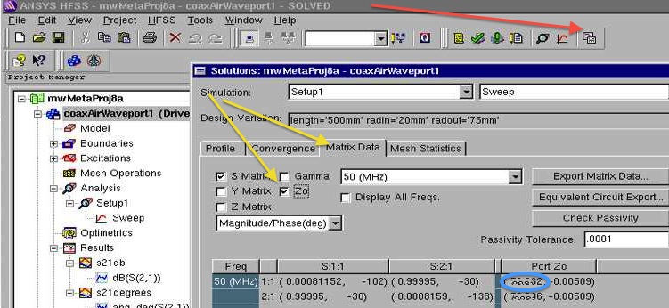
Next, click the solutionsData button (red arrow below)

Select the matrixData tab and check the Zo box (yellow arrows above)
The impedance of the waveport gives the coaxial line impedance. What is the impedance of the coaxial line (blue circle above)? ( Q9 )

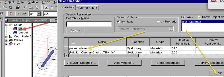
Next, change the coaxial line material in the outer cylinder to polyethylene by right-clicking the "air" material (red arrow below) and selecting "properties"

In the materials popup, select polyethylene and OK (yellow arrows above)
Rerun the simulation as before, but now with the polyethylene dielectric
For the polyethylene coax, save a snapshot of the plot of the angle of S21 in degrees and paste it into your report. ( P3 )
For the polyethylene coax, save a snapshot of the plot of S21 in dB and paste it into your report. ( P4 )
At what frequency is the polyethylene coaxial line section 90 degrees long? ( Q10 )
Is the previous answer the same frequency where the polyethylene line length would equal a quarter wavelength in free-space ? ( Q11 )
Using the same procedure as earlier in this projece, what is the impedance of the polyethylene coaxial cable? ( Q12 )

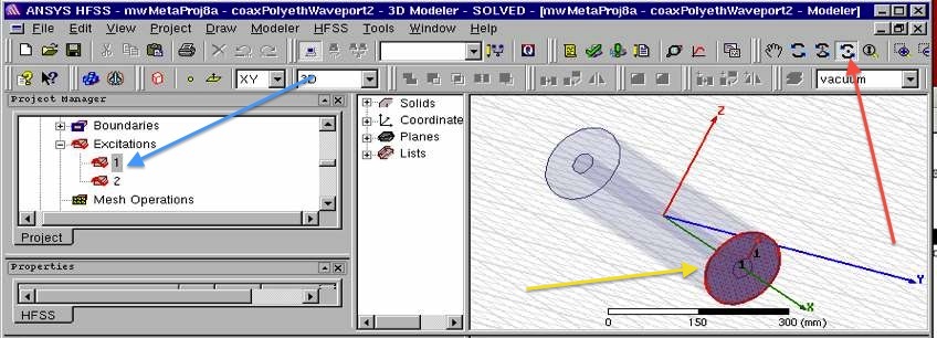
Identify and highlight "waveport 1" (yellow arrow below) by selecting "excitation 1" (blue arrow below)

As shown above, select the rotateAroundScreenCenter button (red arrow above), and reorient the 3D model as shown.
Once you have the model oriented as shown above, and with the "waveport 1" highlighted as shown above, save a snapshot of and paste it into your report. ( P5 )

Exit the program, File->Exit

Part 2

In this part, simulations are performed on a conical monopole antenna using HFSS software.

Although antenna design is not a focus of the course, this simple demo illustrates antenna design capability of the software

Open the second design included in the downloaded project, "conicalMonopole1" (yellow arrow below)

Rerun the simulation as before (yellow circle above)

Plot the radiation pattern (see two blue arrows above), save a snapshot of it, and paste it into your report. ( P6 )

Plot the Smith chart of the antenna input impedance (see two red arrows above), save a snapshot of it, and paste it into your report. ( P7 )

Report

NOTE ReportTemplate: Use the Project Report Template and keep answers to questions on consecutive sheets of paper with all plots at the end.

Do not add extraneous pages or put explanations on separate pages unless specifically directed to do so. The instructor will not read extraneous pages!

Only turn in requested plots (Pxx ) and requested answers to questions (Qxx ). All plots must be labeled P1, P2, etc. and all questions must be numbered Q1, Q2, etc. YOU MUST ADD CAPTIONS AND FIGURE NUMBERS TO ALL FIGURES!!

Cadence, Spectre and Virtuoso are registered trademarks of Cadence Design Systems, Inc., 2655 Seely Avenue, San Jose, CA 95134. Agilent and ADS are registered trademarks of Agilent Technologies, Inc.